Spinning globe with glowing city markers in D3

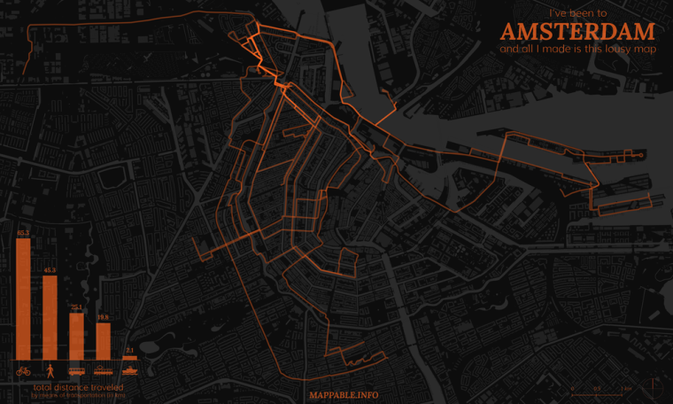
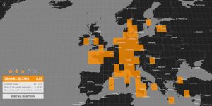
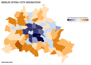
D3 (Data-Driven Documents) is not only one of the currently leading dataviz tool, it also has huge capabilities when it comes to mapping. Here at mappable we’ve so used it for building Travel Score and the Berlin A-Z maps. D3 has a quite steep learning curve, but since I’ve successfully worked with it while only having very basic JavaScript knowledge at that time, it’s definitely doable and in my eyes well worth the effort.


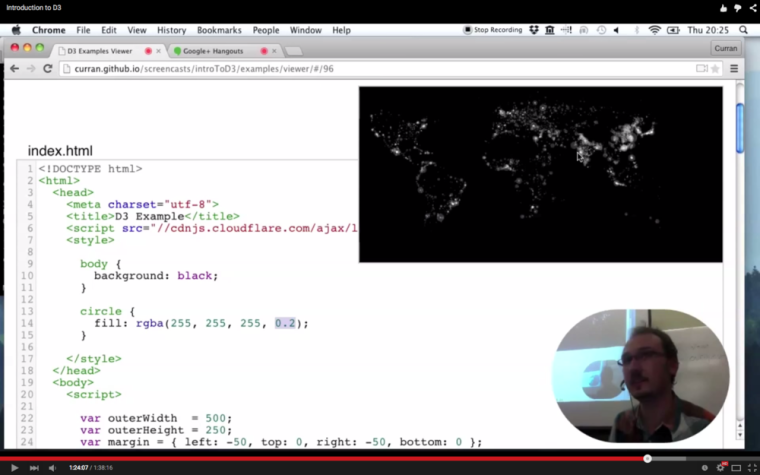
Not having used D3 in quite a while and a little worried that my skills would turn rusty soon, I was pleased to find this tutorial by Curran Kelleher in my twitter feed the other day. It’s a great introduction into D3 and was a welcome opportunity for me to kick start working with D3 again. Close to the end of his tutorial (here), Curran shows how to draw a world map in D3 simply by plotting graduated circle markers according to their lat/long coordinates using Geonames data. I instantly liked the idea and though it would be a good exercise to give the visualization a few additional touches, making use of D3’s extensive mapping functionalities.

First of all, I decided to use D3’s build in orthographic projection. With just a few twists and configurations I had a beautiful globe instead of a flat map. Next, I wanted to get that globe spinning. Why? Basically, because spinning globes are totally fascinating and look awesome! Again, this can be done by adding just a few lines of code.  There’s a great example by Mike Bostock showing the basic principle, which I adopted. Finally, to add some simple interactivity, I’ve integrated some HTML5 sliders and a color picker with the corresponding event listeners.

All together this gives us a spinning globe, showing all cities in the GeoNames databast with a population of more than 100.000 and handlers to manipulate rotation speed & direction, marker opacity, size & color. The result might challenge the rendering capabilities / the processing power of your computer, since it constantly re-calculates and re-projects the positions of over 4.000 markers on the globe. Looking at my machine (a 2013 MacBook Air) that amount is probably at the limit of what you should do with SVG transformations. If you want to build something bigger, working with either canvas or WebGL might be a good idea (see this OpenViz conference talk by Dominikus Bauer for a proper explanation).

Anyway, I’m quite happy with what I’ve build and wanted to share it, since I’ve learned so much just by looking at all the awesome examples out there.

The globe visualization and the source code can be found here or by clicking the image. I decided not to embed it into the blog post, but to use a animated GIF instead, since it could lag or crash browsers on weaker machines. Please also note that the visualization is only optimized for Chrome browsers. I didn’t invest any time in cross-browser compatibility.

Have fun playing with it and happy mapping with D3!

Mapping nightlife

After collecting business listings of relevant categories (nightlife, cinemas, theaters, and event locations) from a popular online directory, the requirements for mapping them were twofold:

  1. The visualizations should allow to identify hot spots of nightlife activity in each city on different map scales.
  2. They should be suitable for comparing the distribution patterns between the different cities.

We chose to tackle this challenge with static dot density maps (sometimes also called dot distribution maps), produced in QGIS. If a data set is large enough, this approach offers a much higher precission than the ordinary choropleth map or any kind of raster or hexbin map that aggregates the data. For the map styling we used cartoDB’s new Dark Matter basemap (finally a project with a good reason to chose the ever so popular dark map style) and plotted all locations on top of it. We set the circle size to 1250 meters and used a very low opacity level as well as the feature blending mode ‘screen’ to highlight those places where a lot of nightlife locations are overlapping.

You can explore the results by either browsing through the gallery on top of this blog post or, if you want to take a closer look at Berlin, Hamburg and Munich check out the high-res, zoomable maps below. As an urban planer it’s fun to see that the nightlife patterns in most cases match to the general city structure (monocentric vs. polycentric) pretty well.

Berlin

Hamburg

Munich

Adding interactivity to static maps

Have you ever been in a situation where you wanted both, a highly individually styled static map and an interactive version at the same time? I recently was and I want to share my experience and my solution in this blog post.

Working as a freelancer, Shenzhen-Jobs.com hired me to produce maps with an individual style, minimum external dependencies, high browser compatibility, and some interactive elements. My approach basically consists of designing individual maps from ground up in QGIS and adding simple interactive elements with Leaflet later on. You can take a look at one of my final maps below. The map’s purpose is to give job seekers, who are unfamiliar with the Shenzhen metropolitan area, a basic understanding of its geography while at the same time showing the spelling of each district in English, Pinyin tone marks and Chinese.

How the map was made:

1. Getting the data
First, I had to download the necessary data sets. Administrative boundaries, streets, train tracks and land use data were downloaded from OpenStreetMap using Geofabrik data extracts & Overpass-Turbo API. Airport locations and coastal boundaries (both mainly used in a larger scale map showing the whole Guangdong region) were downloaded from Natural Earth.

2. Map design in QGIS
All the data sets were loaded into QGIS, individual styling was applied, and labels were added. Having used Adobe Illustrator many times before to give maps a decent finishing, I was really pleased to discover that since version 2.4 QGIS even supports gradient or shapeburst fills. It allows you to create subtle shading of water bodies for example.

3. Exporting static map
The map in its final design was exported as a static file (.jpg and .png both work fine). It’s important to note down the map extents (latitude/longitude), which are displayed in the QGIS print composer.

4. Load static map into Leaflet
I won’t go through the details of making maps with Leaflet – there’s a ton of good examples and tutorials online and it’s really easy to learn by yourself. Loading the static map into Leaflet is done with just three lines of code:

The first line points to the image file, the second passes the map extends on to Leaflet and the third adds the image to the map. Pretty self-explanatory.

5. Adding interactivity with Leaflet
For adding interactivity you need to load more data into the Leaflet map. I’ve exported the district boundaries as GeoJSON with attribute fields for the spelling in the different languages.
Then, the GeoJSON file is loaded via AJAX request using the Leaflet-ajax Plugin by Calvin Metcalf. If you want to know more about how to work with GeoJSON data in Leaflet, read this blog post by Lyzi Diamond.
Once loaded into Leaflet, the Leaflet Label Plugin by Jacob Toye is used to add the labels displaying the different spellings.
To make it even more clear which district the mouse pointer is currently hovering over, I additionally used a highlighting effect, as described by Ben Welsh in this blog post.

In my eyes, this workflow is a nice solution if you need both for a project, static maps and interactivity. Moreover, I’m thrilled that everything necessary to build this map, from the underlying data to the mapping software and the web mapping framework with its plugins, is open source! Feel free to share the map (it’s under CC-BY-NC license) and here’s the source code, in case you want to build something similar:

mapping in deep space

Credit: ESA/Rosetta/NAVCAM, CC BY-SA 3.0 IGO

Landing the fridge-sized probe Philae on 67P/Churyumov-Gerasimenko was without a doubt one of the most fascinating achievements of science and aeronautics this year. We were glued to the screens during the dramatic hours that followed the landing and impressed by the stream of pictures arriving from this distant and unexplored world. The European Space Agency (ESA) did a great job not only with the mission but also by using a Creative Commons License to publish the pictures of the comet.

3d-Mesh of the comet in 123D-Catch

This gave us the possibility to create a 3D-model of the first landing site. Admittedly the ESA published a complete yet low-resolution 3d-model of the comet a few weeks ago but we wanted to try some software anyway: Using 123D Catch from Autodesk we stitched the pictures together and created a meshed and textured *obj file which we then uploaded to Sketchfab. Although not perfect we were impressed by the results. The process is quite simple and we will surely use it on more down-to-earth mapping projects in the future. 

9 days in Amsterdam – Tracking my mobility in bicycle wonderland

As you’ve probably read here before, I (Patrick) am currently on a cartography / dataviz journey around the world. I originally planed to do a lot of mapping during the trip, but didn’t have enough time to do so recently. Too many interesting places to visit and too many short stops so far (which will change soon).

But just after spending 9 days in Amsterdam at the beginning of August, I used the bus ride to Hamburg, and a few more hours later on, for making a map of all my tracks during the stay in Amsterdam. As I didn’t have any special equipment and barely any time to get prepared, this had to work with a very simple approach. If you’re interested in a more sophisticated way of tracking your travels, take a look at Bjørn Sandvik’s blog thematicmapping.

I simply tracked my movement with a smartphone GPS and the OpenPaths service. While I had good experiences with this setup in Germany, it didn’t quite work out abroad. At that time I travelled without a data plan, which meant that my phone couldn’t make use of the A-GPS (Assisted GPS) function, which significantly improves GPS performance. What did that mean for me? Well, a lot of my position data was just useless, the GPS deviations were way too high. But I didn’t want to be stopped by that. Amsterdam and it’s channels (dutch: ‘Grachten’) just look too beautiful on a map to skip this one.

What I ended up doing, was taking the GPS positions as a starting point, made lines out of continuos points and correcting/completing them in QGIS. This took me about two hours, and while the result is not 100% precise, it’s fair enough for a few hours of work and for a first try. The next map of this kind on one of my future stops will be better and the data collection method will improve as well, I promise.

Having complete coverage of my tracks, I categorized the lines according to the means of transportation I’ve used, measured their lengths and added it up to get my personal modal split for my stay in Amsterdam. As you would expect from a city with great bicycle infrastructure, and perfect weather at that time, I ended up using the bike most of the time. For finishing my map, I left QGIS and added the chart and the title in Adobe Illustrator. You can see the final result below, or here in a high-res, zoomable view. And yes, it’s the Netherlands, so it had to be orange/oranje!

Not to forget: the individually designed basemap, with it’s buildings and channels, is based on OpenStreetMap data (© OpenStreetMap contributors), which I’ve extracted via the Overpass API and the XAPI Query Builder. OSM data is available under the Open Database License.

Carsharing time-lapse – Berlin on a World Cup matchday

Last year we released our project ‘one week of carsharing’ for which we analyzed and visualized car2go usage in 19 cities worldwide. Unfortunately we had to take the project offline soon after the release due to a disagreement with Daimler (car2go’s parent company) on our data collection method. As a consequence we thought about a way to present our project without harming Daimler’s interests: simply by showing what we did and how the results look like – this time not with real data but with a synthetic data set for an imaginary city.

In the following weeks and months we got in contact with a lot more people working on carsharing analytics and visualizations from different perspectives (academics, transportation, journalism). One of them was civity management consultants, one of the leading consultancy firms for public services in Europe. They had their own data sets on carsharing usage and asked us to do some cartographic visualizations for them. Their most recent (german) publication is an in-depth analysis of the impact and relevance of ‘free floating carsharing’ – both economically as well as traffic wise.

As a part of our collaboration we had the pleasure to produce a 24h time-lapse video of carsharing activity in Berlin during the day of the World Cup 2014 match Brazil vs. Germany. Take a look at how Berlin is almost standing still during the match (22:00 – 23:45) and how it comes back alive immediately after the victory of the German team. 


The video was produced in Processing and Unfolding with a custom basemap rendered in Tilemill. It was inspired by the project “Seven days of carsharing” by DensityDesign and their Milano time-lapse video. Since it was the first time we worked with Processing and Java code, the release of the visualization’s source code by DensityDesign’s Daniele Ciminieri on github was a huge help for us (Thanks a lot Daniele!).

Basemap data: